R
The Nepaul-Stern Model in R
The Nepaul-Stern Model of Attitude Stability and Constraint is for panel surveys that ask the same people the same attitude questions more than once. The answers are on Likert scales (strongly agree to strongly disagree, liberal–conservative, party identification). Several related attitudes are measured together. Waves may be unevenly spaced, and a person may miss a wave or leave an item blank. Covariates such as age or education can be included.
The questions are about stability (how firmly an attitude persists), constraint (how much one attitude moves with another), how much of the variation comes from lasting individual differences, short-run change, and measurement noise, how a shock to one attitude spreads across later waves, and how covariates relate to the attitudes. Nepaul and Stern (2026) discuss the General Social Survey results. This page is about estimating the model.
Install
You need R 4.0 or newer. On Windows and macOS, CRAN provides a ready-made install, so you do not need a compiler.
install.packages("attitudedyn")
library(attitudedyn)
Linux, and installing without a compiler
On Linux, install.packages("attitudedyn") builds the package on your computer, which needs a C++17 compiler. If you would rather not compile, the Posit Public Package Manager and r2u provide ready-made Linux installs. On the Posit site, choose your distribution and use the repository address it shows. r2u does the same for Ubuntu.
A survey of your own
Put the survey in a data frame with one row per person per wave. id identifies the person and wave identifies the interview. Code each Likert item as the integers 1, 2, 3, and so on, with no skipped code. Leave a skipped item as missing. If someone misses a wave between their first and last interview, keep a row for that wave so the attitude can be carried across it.
For a new sample, use 50 draws. The default is 10, which is what the General Social Survey replication uses. n_threads is how many processors to use. Changing it changes the waiting time. The estimates stay the same. seed = 1 is the default, and it leaves R’s usual random numbers alone.
library(attitudedyn)

# One row per person per wave. Likert items are coded 1, 2, 3, ...
# with no skipped code. Replace the column names with yours.
panel <- read.csv("panel.csv")

fit <- attitudedyn(
  cbind(ideology, party) ~ age + college + female,
  data = panel,
  id = ~ id,
  wave = ~ wave,
  n_factors = 2,
  draws = 50,
  control = attitudedyn_control(n_threads = 4, seed = 1)
)

summary(fit)
persistence_matrix(fit)
impulse_response(fit, horizon = 8)
variance_decomposition(fit)
R adds an intercept for you. Write the formula that way when every row is a real interview. The General Social Survey example below already has an intercept column in the data, and that column is 0 on a wave that was only inserted to fill a gap, so its formula is written 0 + `(Intercept)`.
The General Social Survey example
The numbers below are the printed output from the General Social Survey application in Nepaul and Stern (2026): six Likert items, on the 2006–2020 panels. The items are ideological identification (7 categories), military spending (3), welfare spending (3), the number of immigrants (5), party identification (7), and environmental spending (3). The replication data are on the Harvard Dataverse. The survey file the example reads is gss2.prn. Read it into a data frame named panel, one row per person per wave, with the columns below. The Python package can build that data frame with read_gss().
| Column | What it is |
|---|---|
id, wave | Person and wave. Waves in this file are 1 through 8. No missing values. |
weight | A survey weight, zero or positive, and the same on every row for that person. |
(Intercept), age, hs, college, adv, female, white, black, inc_mid, inc_high | Covariates. The intercept is 1 on a wave that was in the file and 0 on a gap row. |
ideology, military, welfare, immigrants, party, environment | The Likert items, coded from 1. |
Of the 11,282 people in the file, 11,252 have a positive weight and enter the likelihood. Everyone uses the same wave dates, c(2, 3, 4, 5, 6, 7, 8, 10): wave 1 is date 2, and wave 8 is date 10. The gaps are seven steps of 1 and then a step of 2 between the last two waves. Pass that shared grid for this application.
estimates holds the 164 replication starting values, in the order coef() uses. maxit = 0 evaluates that vector and returns. draws = 10 and seed = 1 are the replication defaults: ten simulated paths, each paired with its mirror image (antithetic draws). On 4 threads that evaluation takes a few seconds.
A full search from those starting values took 202.6 seconds on 4 threads. It stopped with convergence code 0 at log-likelihood -111545.0088160454. The tables on this page are the evaluation of the starting values. That log-likelihood is -111570.9702226093, which summary() prints as -111571.
fit <- attitudedyn(
  cbind(ideology, military, welfare, immigrants, party, environment) ~
    0 + `(Intercept)` + age + hs + college + adv + female + white + black +
    inc_mid + inc_high,
  data = panel,
  id = ~ id,
  wave = ~ wave,
  time_grid = c(2, 3, 4, 5, 6, 7, 8, 10),
  weights = weight,
  n_factors = 2,
  draws = 10,
  start = unname(estimates),
  control = attitudedyn_control(
    maxit = 0,
    n_threads = 4,
    vcov = "opg_centered",
    seed = 1
  )
)
Then read the fit. The small draw count in predict() is only the setting that produced the printed excerpt. In your own work, leave n_draws at its default, which is at least 20.
summary(fit)
glance(fit)
tidy(fit)
persistence_matrix(fit)
irf <- impulse_response(fit, horizon = 8)
irf$spectral_radius
variance_decomposition(fit)
head(predict(fit, type = "class", n_draws = 2, seed = 2))
head(predict(fit, type = "prob", n_draws = 2, seed = 2)$ideology)
head(simulate(fit, nsim = 1, seed = 2))
Summary
summary(fit) opens with the sample size and the log-likelihood, then prints every free coefficient. There are 164 of them. glance(fit) is one row of fit statistics. tidy(fit) is the coefficient table as a data frame. These are the opening lines, the one-row summary, and the first rows of tidy(fit) (the ideology wave effects).
Dynamic ordinal attitude model
Log-likelihood: -111571
People: 11252   Attitudes: 6   Waves: 8
Draws: 10 (plus antithetic twins)
Free coefficients: 164
Converged. logLik AIC BIC nobs n_free draws converged
1 -111571 223469.9 224671.8 11252 164 10 TRUE term estimate std.error statistic p.value
1 wave_effect[ideology,1] 2.194142 0.05376410 40.81055 0.000000e+00
2 wave_effect[ideology,2] 2.074462 0.05245524 39.54728 0.000000e+00
3 wave_effect[ideology,3] 2.027419 0.05290115 38.32467 0.000000e+00
4 wave_effect[ideology,4] 1.923106 0.05950472 32.31854 3.840033e-229
5 wave_effect[ideology,5] 1.826457 0.06550899 27.88101 4.534093e-171
6 wave_effect[ideology,6] 2.086153 0.05284053 39.48018 0.000000e+00
7 wave_effect[ideology,7] 2.066090 0.05334925 38.72763 0.000000e+00
8 wave_effect[ideology,8] 2.056632 0.05238561 39.25949 0.000000e+00Persistence and impulse responses
persistence_matrix() is on a scale from −1 to 1. The row is the attitude that receives the past. The column is the attitude that is lagged. summary() prints that matrix rounded to three decimals. The function itself prints more digits.
impulse_response() follows a one-unit shock. Horizon 0 is the shock itself. Later rows are the response after that many steps. For this fit the spectral radius is 0.636678. The figure is the same grid: rows respond, columns are the shock. Nepaul and Stern (2026) discuss what the paths mean.
Persistence on (-1, 1), receiving attitude by source attitude:
            ideology military welfare immigrants  party environment
ideology       0.242   -0.033  -0.033      0.043 -0.146      -0.101
military      -0.015    0.503   0.003      0.017 -0.086       0.012
welfare       -0.003    0.031   0.536      0.009  0.053      -0.157
immigrants     0.010    0.009   0.050      0.434  0.057      -0.132
party         -0.233   -0.079   0.028      0.039  0.467      -0.036
environment   -0.120    0.007  -0.031     -0.116  0.000       0.281

Covariance type: opg_centered ideology military welfare immigrants party
ideology 0.241617418 -0.033489725 -0.032641594 0.042786144 -0.1464621228
military -0.014958273 0.503399564 0.002622063 0.016527763 -0.0859475246
welfare -0.002560862 0.031288136 0.536315888 0.009337382 0.0534814626
immigrants 0.009940252 0.008915214 0.050386823 0.434174577 0.0573418470
party -0.233068940 -0.078857718 0.027697333 0.038619875 0.4673942578
environment -0.120417498 0.006960558 -0.030590966 -0.116273026 -0.0002142674
environment
ideology -0.10082475
military 0.01190907
welfare -0.15660637
immigrants -0.13201325
party -0.03608537
environment 0.28139499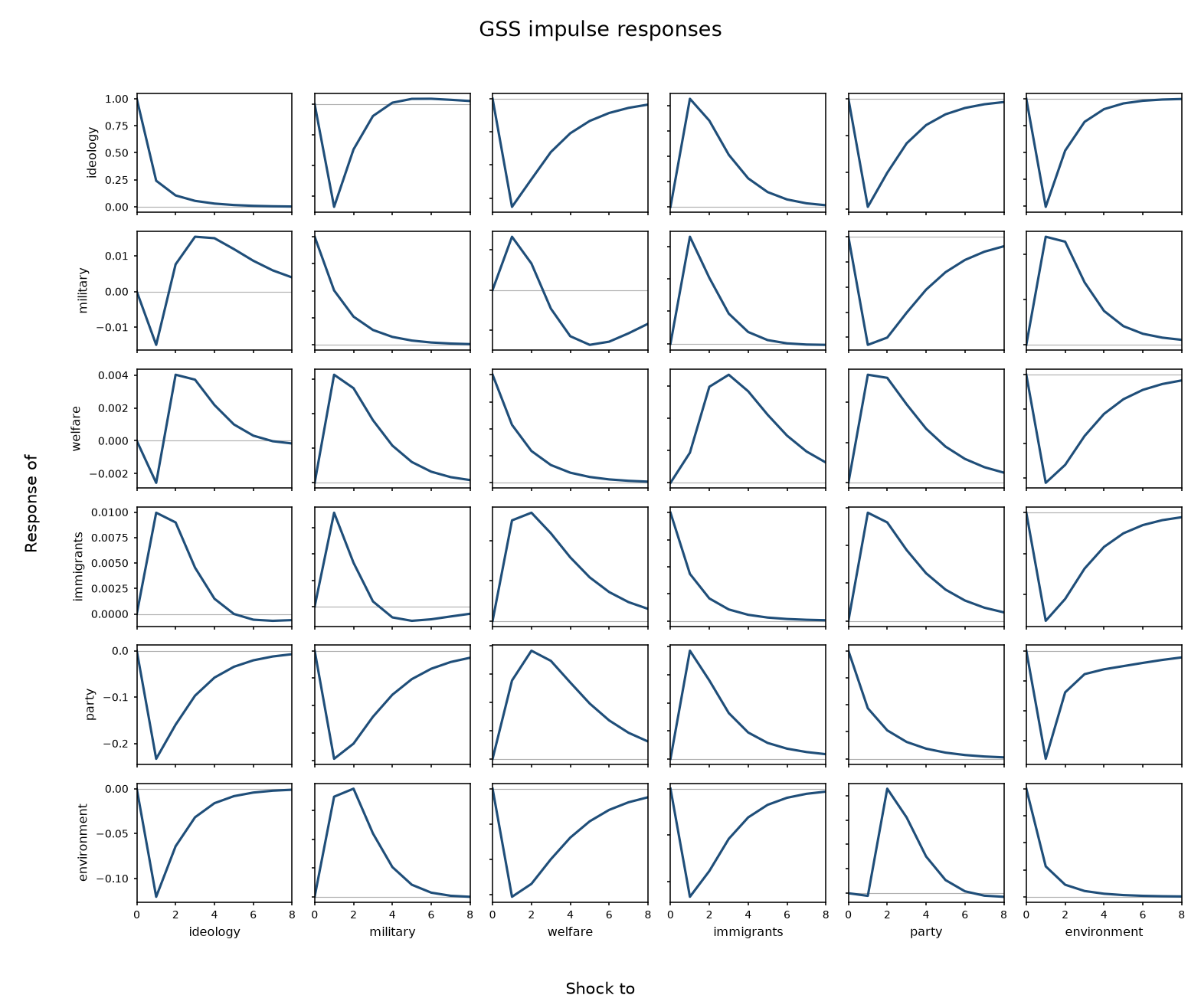
Variance decomposition
variance_decomposition() reports four pieces for each latent attitude. covariate is the variance of the wave effect plus the covariates. wave_effect is the wave effect on its own. factor is the sum of squared loadings, the part that stays with the person across waves. shock is the average short-run contribution built from the persistence coefficients. total adds the four.
     attitude  covariate wave_effect    factor    shock    total
1    ideology 0.05539829 0.006743936 1.0157923 1.075184 2.153119
2    military 0.08066210 0.012030993 0.2563862 1.230515 1.579594
3     welfare 0.06768285 0.008042642 0.3143057 1.281257 1.671288
4  immigrants 0.11566266 0.025941273 0.1506216 1.180127 1.472352
5       party 0.15248945 0.008187262 1.6801225 1.241410 3.082209
6 environment 0.08822739 0.044159354 0.5093202 1.087319 1.729025
Predicted categories and a new panel
predict(..., type = "class") is the Likert category with the highest probability. type = "prob" is the probability of each category. The excerpt below is ideology. The row numbers skip, because they are positions in the person-by-wave array and waves outside a person’s window are still in that array.
simulate() draws a new panel from the fitted coefficients, with 11,252 people and 8 waves (90,016 rows). The intercept column is ones. The other covariates are standard normal. The seed used for the printed rows is 2.
    id wave ideology military welfare immigrants party environment
1  1001    1        4        1       2          1     1           3
2  1001    2        4        1       1          3     1           3
3  1001    3        4        1       1          3     1           3
9  1002    1        2        1       3          3     1           3
10 1002    2        2        1       3          3     1           3
11 1002    3        4        1       2          3     1           3
17 1003    1        4        2       3          1     1           3
18 1003 2 4 2 3 1 1 3 id wave p1 p2 p3 p4 p5 p6
1 1001 1 0.02758044 0.1272366 0.1272589 0.3648183 0.15185606 0.17056472
2 1001 2 0.03794270 0.1439802 0.1227266 0.2988741 0.13858043 0.20433331
3 1001 3 0.03870095 0.1463892 0.1263869 0.3213133 0.14303027 0.18459334
9 1002 1 0.16961015 0.3121439 0.1900333 0.2799786 0.03572320 0.01219481
10 1002 2 0.20219138 0.3195043 0.1820723 0.2555146 0.03056457 0.00991825
11 1002 3 0.13838390 0.2846763 0.1878729 0.3175696 0.05049026 0.02031592
p7
1 0.0306849530
2 0.0535626919
3 0.0395860755
9 0.0003160778
10 0.0002345712
11 0.0006911060 id wave time `(Intercept)` age hs college adv
1 1 1 2 1 -0.9026492 0.50903832 0.2301757 1.20352629
2 1 2 3 1 0.4938905 0.63569010 1.4042788 0.57787148
3 1 3 4 1 1.1721555 0.04787437 -1.5068600 0.02361624
4 1 4 5 1 -1.1126723 -0.07966583 -0.2856974 -1.33421211
5 1 5 6 1 0.4599354 0.99818882 -1.0672768 1.54923301
6 1 6 7 1 -0.4065013 0.70675225 -0.3270731 -0.84974658
female white black inc_mid inc_high ideology military
1 -1.0757920 1.4073684 0.8245715 1.3188503 0.08765931 4 1
2 -0.5703429 -0.6362407 -0.7278699 0.7104078 -0.42438204 4 1
3 -1.0646881 -0.7731621 0.7288264 1.4819691 -1.14535413 4 1
4 -0.5488183 -1.3743841 -0.8756520 -1.3382348 0.86257042 4 1
5 -0.1009926 -1.1099300 -0.7438604 -0.9587655 -1.20854974 4 1
6 -0.8482505 1.1923700 -1.1455800 0.8882187 1.06460981 5 2
welfare immigrants party environment
1 3 1 3 3
2 2 5 2 3
3 3 2 1 2
4 3 3 2 2
5 3 5 1 2
6 3 3 6 3The corner of the stored covariance matrix
summary() uses the covariance stored with the fit. Here that is opg_centered. This is the corner of that matrix.
                        wave_effect[ideology,1] wave_effect[ideology,2]
wave_effect[ideology,1]                0.002891                0.002241
wave_effect[ideology,2]                0.002241                0.002752
wave_effect[ideology,3]                0.002252                0.002404
                        wave_effect[ideology,3]
wave_effect[ideology,1]                0.002252
wave_effect[ideology,2]                0.002404
wave_effect[ideology,3]                0.002799
How it works, briefly
The arithmetic is done by a C++17 program that has no libraries of its own. The R package calls that program.
The likelihood is simulated, by the Geweke–Hajivassiliou–Keane (GHK) method. The slope of the likelihood is analytic, and the search uses BFGS.
The random draws use Philox. Each draw is tied to the seed, the person, and the draw number, so the same data and seed give the same answer with any number of threads, and on Windows, macOS, and Linux.
The loop over people can use several threads. Standard errors can be the outer product of the person-level scores (the default, opg_centered, or the uncentred opg), the curvature of the likelihood (hessian), or the sandwich combination of those two.
For the substantive reading of a set of estimates, including the General Social Survey application, see Nepaul and Stern (2026).